Adding Objects to the Viewer

Off the bat Octarine supports 6 types of objects, all of which have dedicated Viewer methods:

	Object Type	Viewer method
1.	Meshes	octarine.Viewer.add_mesh
2.	Points	octarine.Viewer.add_points
3.	Lines	octarine.Viewer.add_lines
4.	Image Volumes	octarine.Viewer.add_volume
5.	Sparse Volumes	octarine.Viewer.add_sparse_volume
6.	Tubes	octarine.Viewer.add_tubes

As a general entry point you can use the octarine.Viewer.add() method which will pass an object to the respective specialized function:

>>> v = oc.Viewer()
>>> # This ...
>>> v.add(mesh)
>>> # ... is effectively the same as this
>>> v.add_mesh(mesh)

Tip

The specialised methods may offer more ways to customize the visual.

Meshes

Octarine will happily work with anything that's mesh-like - i.e. anything that has .vertices and .faces. In practice, I'd recommend you use trimesh to e.g. load meshes from files:

>>> import octarine as oc
>>> import trimesh as tm

>>> mesh = tm.load_remote(
...         'https://github.com/mikedh/trimesh/raw/main/models/bunny.ply'
...     )
>>> type(mesh)
<trimesh.Trimesh(vertices.shape=(8146, 3), faces.shape=(16301, 3), name=`bunny.ply`)

>>> v = oc.Viewer()
>>> v.add_mesh(mesh, name='bunny')

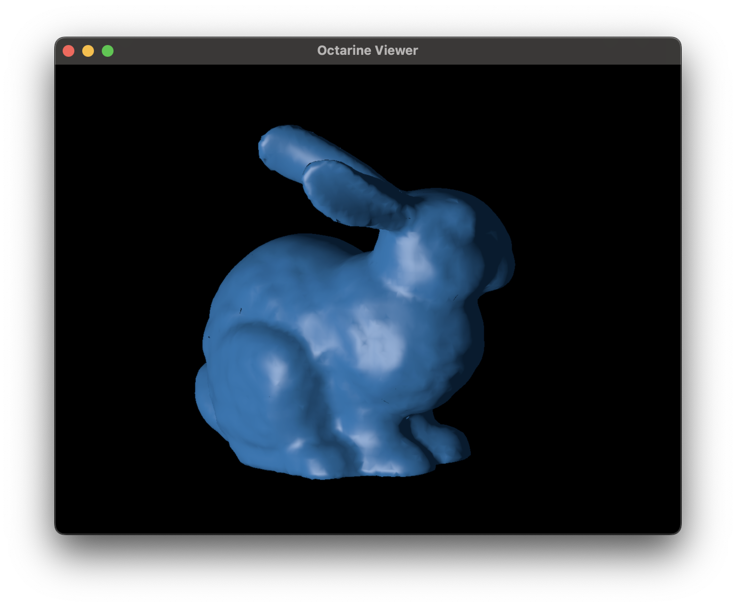
See octarine.Viewer.add_mesh() for details!

Points

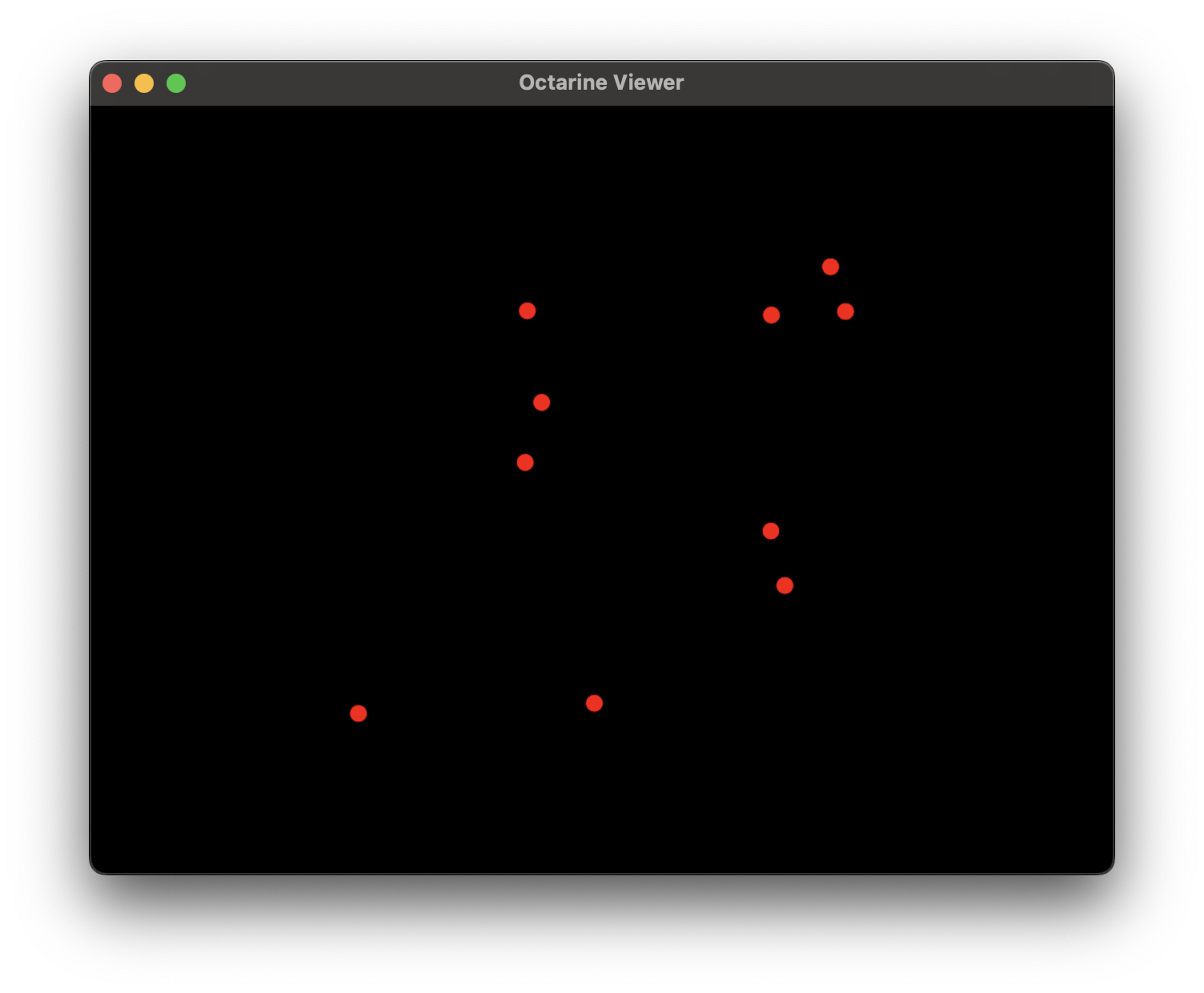
Points are expected to be 2d (N, 3) numpy arrays:

>>> import octarine as oc
>>> v = oc.Viewer()

>>> # Add random points as scatter
>>> import numpy as np
>>> points = np.random.rand(10, 3)  # 10 random points
>>> v.add_points(points, color='r')

Markers, sizes and edges

By default, points are rendered as simple squares with a constant on-screen size. Both of these things can be customized:

>>> v.add_points(
...     points,
...     marker='ring',             # see pygfx.MarkerShape for options
...     size=500,                  # size in world units ...
...     size_space='world',        # ... i.e. markers scale when you zoom
...     min_size=5,                # but keep them at least 5 pixels on screen
...     edge_color='black',        # give the markers ...
...     edge_width=2,              # ... a black edge
...     edge_size_space='screen',  # edge width stays constant on screen
... )

A couple notes on the above:

• marker accepts the shapes in pygfx.MarkerShape - e.g. "circle", "ring", "diamond", "cross" or "pin"
• size can be a single value or an array with one size per point
• with size_space="world" (or "model"), size is the marker's diameter in world (model) units; the default "screen" keeps sizes constant in on-screen pixels
• min_size/max_size clamp the on-screen size (in logical pixels): "500 world units but at least 5 pixels" keeps far-away points visible
• edge_mode controls whether the edge is drawn "inner", "outer" or "centered" (default) relative to the marker's outline

Some of these options (e.g. min_size/max_size or an edge width in units different from the marker size) are powered by a custom shader which requires pygfx>=0.17; unless one of them is used, Octarine sticks with the stock pygfx materials.

See octarine.Viewer.add_points() for details!

Lines

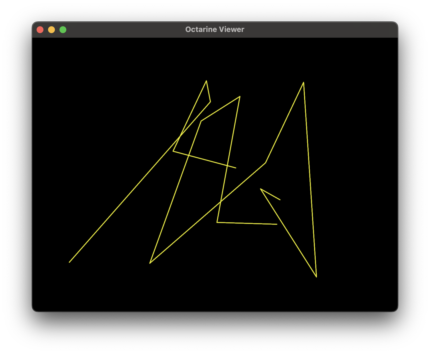
Lines are expected to be either a (N, 3) numpy array representing a single contiguous line or a list thereof:

>>> import octarine as oc
>>> v = oc.Viewer()

>>> import numpy as np
>>> line1 = np.random.rand(10, 3)  # points for line 1
>>> line2 = np.random.rand(5, 3)  # points for line 2
>>> v.add_lines([line1, line2], color='y')

See octarine.Viewer.add_lines() for details!

Image Volumes

Image volumes are expected to be 3d numpy arrays or trimesh.VoxelGrids.

In this example, we're using pynrrd to read an image stack of a Drosophila brain downloaded from figshare (link):

>>> import nrrd
>>> vol, meta = nrrd.read('JRC2018_UNISEX_38um_iso_16bit.nrrd')
>>> # Dimensions along each axis are 0.38 microns
>>> meta['sizes']
array([[0.38, 0.  , 0.  ],
       [0.  , 0.38, 0.  ],
       [0.  , 0.  , 0.38]])

>>> import octarine as oc
>>> v = oc.Viewer()
>>> v.add_volume(vol, spacing=(.38, .38, .38))
>>> v.show_bounds = True

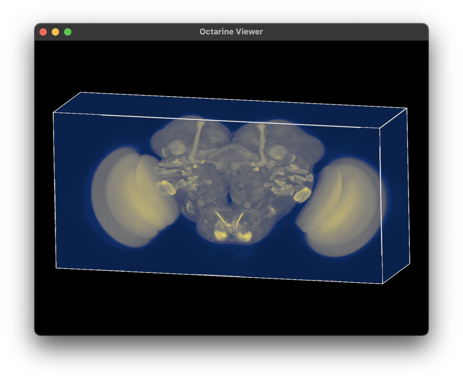
Note that the default blend mode for the renderer may cause objects behind or inside the volume to look funny. You can change the blend mode by setting e.g. v.set_alpha_mode('add') - see Effects & Shading for details.

Alternatively, you can also add slices through the volume:

>>> import cmap
>>> v.add_volume(
...     vol,
...     color=cmap.Colormap('Greys'),  # use a different colormap
...     spacing=.38,  # single value for isometric data
...     slice=True  # can also be a tuple, e.g. (True, False, True)
... )

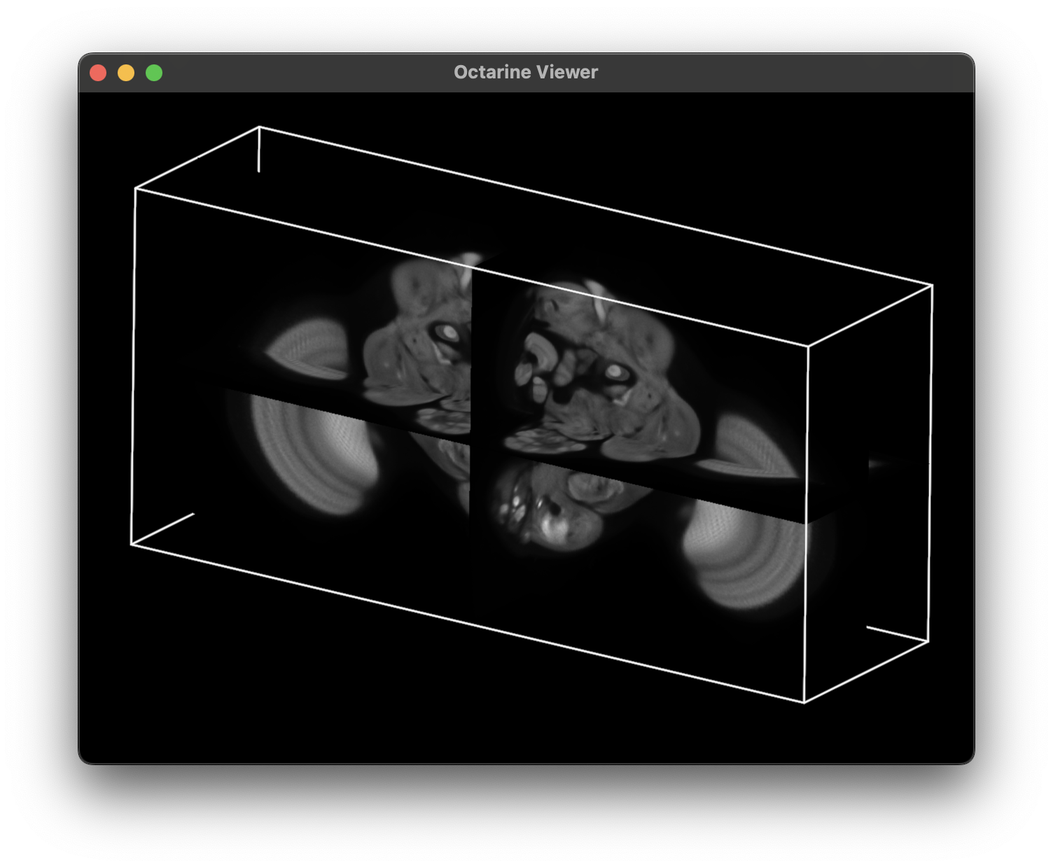
See octarine.Viewer.add_volume() for details!

Sparse Volumes

Image volumes work great for dense data but if your data is sparse - e.g. a segmentation mask or a cloud of voxels - building a dense 3D grid can be prohibitively expensive. For that, Octarine offers octarine.Viewer.add_sparse_volume(): instead of a 3D grid it accepts an (N, 3) array of voxel coordinates (plus optional per-voxel values) which is rendered with a custom raycasting shader. Its memory footprint scales with the number of occupied 16³ bricks rather than with the bounding box, so tens of millions of voxels are feasible:

>>> import numpy as np
>>> import octarine as oc

>>> # Generate some sparse voxel coordinates (a hollow sphere)
>>> phi = np.random.rand(1_000_000) * 2 * np.pi
>>> costheta = np.random.rand(1_000_000) * 2 - 1
>>> theta = np.arccos(costheta)
>>> voxels = np.stack([
...     np.sin(theta) * np.cos(phi),
...     np.sin(theta) * np.sin(phi),
...     np.cos(theta)
... ], axis=1) * 500

>>> v = oc.Viewer()
>>> v.add_sparse_volume(voxels)

Useful parameters:

• values: per-voxel scalars mapped onto the colormap; without them the volume is rendered as binary occupancy
• mode: "mip" (maximum-intensity projection; default), "density" (cloud-like front-to-back emission/absorption) or "surface" (see below)
• spacing / offset: voxel side lengths and world offset
• clim: (min, max) range used to scale values
• step_size: ray-march step in voxels - smaller values miss fewer small structures but render slower

Surface rendering

mode="mip" and mode="density" have no notion of a surface: for binary occupancy data every ray that hits anything returns the same value, so the volume reads as a flat, homogeneous blob. mode="surface" instead stops at the first isosurface crossing and shades it using the gradient of the volume as the surface normal, which is what makes the shape legible:

>>> v.add_sparse_volume(voxels, mode="surface")

• threshold (default 0.5) sets the level at which the surface sits, as a fraction of clim. For binary occupancy the default puts it halfway between an empty and a full voxel; with values it selects an iso-level
• lighting is a fixed headlight, so the surface is always lit from the front

Because the normal is derived from the volume itself, binary data - whose values jump from 0 to 1 over a single voxel - gives somewhat faceted normals. The material exposes a few knobs to tune this:

>>> vis = v["SparseVolume.1"][0]
>>> vis.material.gradient_delta = 1.5  # smoother normals, rounder features
>>> vis.material.shininess = 5         # duller specular highlight
>>> vis.material.emissive = "#202020"  # lift the unlit side

gradient_delta is the half-width (in voxels) of the differences the normal is derived from. Raising it smooths the voxel staircase on solid, blobby data but only up to a point: features thinner than the delta fall between the two samples, which flattens their shading. Keep it at the default of 1 for thin structures such as segmentation shells or skeletons.

Note that interpolation="nearest" in surface mode snaps the normals to the voxel axes, which gives a deliberately blocky, Minecraft-like look.

Smoothing

Zoomed in far enough, an isosurface through binary data shows a fine voxel-scale stipple: the trilinear filter the normal is taken from only reaches one voxel, so the normal tracks individual voxel faces. The smoothing parameter widens that filter only:

>>> v.add_sparse_volume(voxels, mode="surface", smoothing=1.5)

It is given in voxels; 0 (the default) is off and 1-2 is usually enough. The isosurface itself stays on the unsmoothed field, so the silhouette comes out pixel-identical and no thin structures are lost - only the shading changes. On a 31M-voxel neuron it costs ~4% at close zoom.

Why not smooth the surface as well?

Because a wider filter shrinks a binary volume. A feature only reaches full value while it is thicker than 2 + 2 * smoothing voxels; below that its peak drops away and the isosurface breaks up. At smoothing=1.5 a 2-voxel-thick neurite peaks at 0.51 - right at the default threshold. Filtering the normal alone sidesteps that entirely, and on real data it looks the same, since it is the shading rather than the silhouette that carries the voxel look.

smoothing pairs with gradient_delta: a difference much narrower than the filter reads nearly the same value at both taps and yields noise rather than a direction. The shader therefore widens the stencil along with the filter, so gradient_delta only takes effect once it exceeds 0.5 + smoothing.

Density rendering

In mode="density" the volume is accumulated front-to-back, so thicker parts render more opaque. The density parameter (default 0.1) is the extinction per voxel at the top of clim: raise it for a more solid look, lower it for a wispier one. - method: "auto" (default) uses the custom shader and falls back to binning into a (downsampled) dense grid if the data occupies too many bricks

Run-length encoded voxels

add_sparse_volume also accepts run-length encoded voxels as an (N, 4) array of (x, y, z, x_run_length) - the layout DVID's sparsevol endpoint returns:

>>> import dvid
>>> runs = dvid.get_sparsevol(bodyid, scale=2, voxels=False)   # (N, 4)
>>> v.add_sparse_volume(runs, mode="surface")

Runs take a different path through the shader. Coordinates are packed into a byte-per-voxel atlas that can carry per-voxel values; runs are packed into a bit-per-voxel bitmask, which is binary occupancy only but uses roughly 23x less GPU memory. On a 31M-voxel DVID neuron:

	GPU memory	bytes/voxel
(N, 3) coordinates (byte-per-voxel atlas)	328 MB	10.5
(N, 4) runs (bit-per-voxel bitmask)	14 MB	0.45

Passing values alongside runs raises an error - there is nowhere to put them. If you have binary (N, 3) coordinates and want the same saving, pass method="bitmask" and they will be converted to runs for you.

Note that runs never need expanding: the packer consumes the (N, 4) array directly, so a neuron that would be 376 MB as (N, 3) int32 coordinates never materializes.

You can also wrap the coordinates in a octarine.VoxelCloud (or runs in a octarine.VoxelRuns) - this tells the generic Viewer.add to route them to the sparse-volume pipeline (a plain (N, 3) array would be interpreted as points):

>>> from octarine import VoxelCloud, VoxelRuns
>>> v.add(VoxelCloud(voxels))
>>> v.add(VoxelRuns(runs))

Note that sparse volumes require pygfx>=0.17.

See octarine.Viewer.add_sparse_volume() for details!

Tubes

Skeletons with a varying, non-circular cross-section - neuronal arbors, vessels, streamlines - can be drawn as tubes without ever building a mesh. octarine.Viewer.add_tubes() takes a per-node radial profile

$$r(\theta) = a_0 + \sum_k \left[ a_k \cos(k\theta) + b_k \sin(k\theta) \right]$$

and generates the whole surface in the vertex shader. Each node is 8 + 2K floats - position, a frame quaternion, the mean radius a0, then K cosine and K sine coefficients - plus an (E, 2) edge list. At K = 4 that is 64 bytes a node, whatever resolution you draw it at:

>>> import numpy as np
>>> import octarine as oc

>>> # A straight tube along +x with an elliptic cross-section
>>> n, K = 50, 2
>>> coefs = np.zeros((n, 8 + 2 * K), dtype=np.float32)
>>> coefs[:, 0] = np.linspace(0, 100, n)      # positions
>>> coefs[:, 3:7] = (0.5, 0.5, 0.5, 0.5)      # frame (u, v, t) = (+y, +z, +x)
>>> coefs[:, 7] = 5                           # mean radius a0
>>> coefs[:, 9] = 2                           # a_2: make it elliptic
>>> edges = np.column_stack([np.arange(n - 1), np.arange(1, n)])

>>> v = oc.Viewer()
>>> v.add_tubes(coefs, edges=edges)

Useful parameters:

• axial_lod: axial level of detail. 0 is full resolution, 1 keeps every 2nd node, 2 every 4th, and so on. Branch points and tips are always kept, so no arm can go missing. A cost lever rather than a quality one
• n_theta: number of angular samples around the tube. This is the angular level of detail - 32 is smooth, 8 still gives a reasonable silhouette at a quarter of the vertices
• k: number of harmonics to evaluate for the surface position; 0 renders circular tubes of radius a0
• k_normal: number of harmonics to evaluate for the normal (default 1, clamped to k) - see the note below
• color: a single color, or an (M, 3)/(M, 4) array for per-node colors
• offset: world offset (node positions are expected in physical units, so there is no spacing)

Self-intersection

The tube surface is generated in the vertex shader by sweeping the cross-section along the skeleton. It is cheap - the cost is per vertex, and a coarse n_theta makes it cheaper still - and the silhouette is exactly the profile you gave it.

Its one failure mode is inherent to sweeping: a swept surface folds through itself wherever the cross-section radius outruns the centreline's local radius of curvature. Skeletons traced from voxel data routinely violate that, since node spacing is typically ~1 voxel while radii are several, so a little positional jitter tilts consecutive rings into one another. The result looks like a pile of intersecting discs - the classic "why does my tube look like a crappy mesh".

There is currently no good fix for this, and the ones that look obvious have been tried and reverted - a raycast union of solids, low-passing the centreline, and sweeping each edge as a C2 cubic B-spline rather than a straight interpolation. All three improved the self-intersection metrics; none visibly improved the render. See "What has been tried" in octarine.shaders.tubes before attempting a fourth, because the evidence points at the angular profile rather than the sweep: adjacent nodes' harmonic magnitudes differ by 50-65%, so consecutive cross-sections are genuinely different shapes.

The one lever that does help today is dropping harmonics, which trades silhouette fidelity for a much cleaner surface:

>>> v.add_tubes(coefs, edges=edges, k=3)

axial_lod also reduces self-intersection, but weakly and at a steep price in axial detail - it drops the nodes carrying it, and boutons and varicosities are a local bump in a0 along the axis. Treat it as a vertex-cost knob.

Why k_normal defaults lower than k

The surface normal comes from dr/dθ, which weights harmonic k by k. Once the harmonic magnitudes flatten out at the resolution floor of the data - which they typically do, with no clear knee - every extra harmonic contributes more slope than shape: the silhouette keeps improving while the shading gets noisier, until the normal tilts far enough past the view direction to leave dark patches. Truncating the normal at k_normal=1 (or 0 for a perfectly smooth tube) keeps the full silhouette and drops the sandpaper. Raise it only if you want the roughness.

Both n_theta and k are uniforms, so changing them re-draws at a different resolution without touching the coefficient buffer:

>>> vis = v.objects["Tubes"][0]
>>> vis.material.n_theta = 8     # no upload, no reallocation
>>> vis.material.k_normal = 0    # ... and so is smoothing the shading

Axial detail is not free in quite the same way: dropping nodes means a different edge list. That is still only a small index buffer - pass a decimated edges array while the coefficients stay as they are.

add_tubes also accepts anything that quacks like a sparsecubes.TubeProfile (i.e. has a0, mag, phase, frame, edges and to_gpu_buffer()), in which case the coefficients and edges are pulled off the object - and Viewer.add routes such objects here automatically:

>>> v.add(profile)

Note that tubes require pygfx>=0.17.

See octarine.Viewer.add_tubes() for details!

Custom Objects

What if you have want to visualize something not currently supported by Octarine?

Go check out the Extending Octarine tutorial to learn how!

What next?

• Animations

  ---

  Add movement to the viewer.

  Animations

• Control

  ---

  Learn how to control the viewer, adjust colors, etc.

  Controls